Ferrotec Nord’s Thermoelectric Technical Reference Guide is a comprehensive technical explanation of thermoelectrics and thermoelectric technology.
9.0 Thermoelectric module selection
9.1 Selection of the proper TE Cooler for a specific application requires an evaluation of the total system in which the cooler will be used. For most applications it should be possible to use one of the standard module configurations while in certain cases a special design may be needed to meet stringent electrical, mechanical, or other requirements. Although we encourage the use of a standard device whenever possible, Ferrotec America specializes in the development and manufacture of custom TE modules and we will be pleased to quote on unique devices that will exactly meet your requirements.
The overall cooling system is dynamic in nature and system performance is a function of several interrelated parameters. As a result, it usually is necessary to make a series of iterative calculations to «zero-in» on the correct operating parameters. If there is any uncertainty about which TE device would be most suitable for a particular application, we highly recommend that you contact our engineering staff for assistance.
Before starting the actual TE module selection process, the designer should be prepared to answer the following questions:
- At what temperature must the cooled object be maintained?
- How much heat must be removed from the cooled object?
- Is thermal response time important? If yes, how quickly must the cooled object change temperature after DC power has been applied?
- What is the expected ambient temperature? Will the ambient temperature change significantly during system operation?
- What is the extraneous heat input (heat leak) to the object as a result of conduction, convection, and/or radiation?
- How much space is available for the module and heat sink?
- What power is available?
- Does the temperature of the cooled object have to be controlled? If yes, to what precision?
- What is the expected approximate temperature of the heat sink during operation? Is it possible that the heat sink temperature will change significantly due to ambient fluctuations, etc.?
Each application obviously will have its own set of requirements that likely will vary in level of importance. Based upon any critical requirements that can not be altered, the designer’s job will be to select compatible components and operating parameters that ultimately will form an efficient and reliable cooling system. A design example is presented in section 9.5 to illustrate the concepts involved in the typical engineering process.
9.2 USE OF TE MODULE PERFORMANCE GRAPHS: Before beginning any thermoelectric design activity it is necessary to have an understanding of basic module performance characteristics. Performance data is presented graphically and is referenced to a specific heat sink base temperature. Most performance graphs are standardized at a heat sink temperature (Th) of +50°C and the resultant data is usable over a range of approximately 40°C to 60°C with only a slight error. Upon request, we can supply module performance graphs referenced to any temperature within a range of -80°C to +200°C.
9.3 To demonstrate the use of these performance curves let us present a simple example. Suppose we have a small electronic «black box» that is dissipating 15 watts of heat. For the electronic unit to function properly its temperature may not exceed 20°C. The room ambient temperature often rises well above the 20°C level thereby dictating the use of a thermoelectric cooler to reduce the unit’s temperature. For the purpose of this example we will neglect the heat sink (we cannot do this in practice) other than to state that its temperature can be maintained at 50°C under worst-case conditions. We will investigate the use of a 71-couple, 6-ampere module to provide the required cooling.
9.3.1 GRAPH: Qc vs. I This graph, shown in Figure (9.1), relates a module’s heat pumping capacity (Qc) and temperature difference (DT) as a function of input current (I). In this example, established operating parameters for the TE module include Th = 50°C, Tc = 20°C, and Qc = 15 watts. The required DT = Th-Tc = 30°C.
It is necessary first to determine whether a single 71-couple, 6-ampere module is capable of providing sufficient heat removal to meet application requirements. We locate the DT=30 line and find that the maximum Qc value occurs at point A and with an input current of 6 amperes. By extending a line from point A to the left y-axis, we can see that the module is capable of pumping approximately 18 watts while maintaining a Tc of 20°C. Since this Qc is slightly higher than necessary, we follow the DT=30 line downward until we reach a position (point B) that corresponds to a Qc of 15 watts. Point B is the operating point that satisfies our thermal requirements. By extending a line downward from point B to the x-axis, we find that the proper input current is 4.0 amperes.
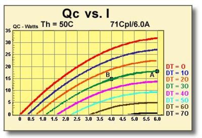
Figure (9.1) Heat pumping capacity related to temperature differential as a function of input current for a 71-Couple, 6-Ampere Module
9.3.2 GRAPH: Vin vs. I This graph, shown in Figure (9.2), relates a module’s input voltage (Vin) and temperature difference (DT) as a function of input current (I). In this example, parameters for the TE module include Th = 50°C, DT = 30°C, and I = 4.0 amperes. We locate the DT=30 line and, at the 4.0 ampere intersection, mark point C. By extending a line from point C to the left y-axis, we can see that the required module input voltage (Vin) is approximately 6.7 volts.
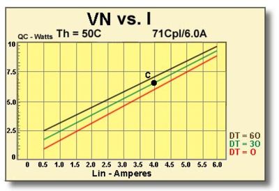
Figure (9.2) Input voltage related to temperature differential as a function of input current for a 7I-Couple, 6-Ampere Module
9.3.3 GRAPH:COP vs. I This graph, shown in Figure (9.3), relates a module’s coefficient of performance (COP) and temperature differential (DT) as a function of input current (I). In this example, parameters for the TE module include Th = 50°C, DT = 30°C, and I = 4.0 amperes.
We locate the DT=30 line and, at the 4.0 ampere intersection, mark point D. By extending a line from point D to the left y-axis, we can see that the module’s coefficient of performance is approximately 0.58.
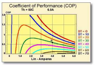
Figure (9.3) Coefficient of performance related to temperature differential as a function of input current for a 71-Couple, 6-Ampere Module
Note that COP is a measure of a module’s efficiency and it is always desirable to maximize COP whenever possible. COP may be calculated by:
9.4 An additional graph of Vin vs. Th, of the type shown in Figure (9.4), relates a module’s input voltage (Vin) and input current (I) as a function of module hot side temperature (Th). Due to the Seebeck effect, input voltage at a given value of I and Th is lowest when DT=O and highest when DT is at its maximum point. Consequently, the graph of Vin vs. Th usually is presented for a DT=30 condition in order to provide the average value of Vin.
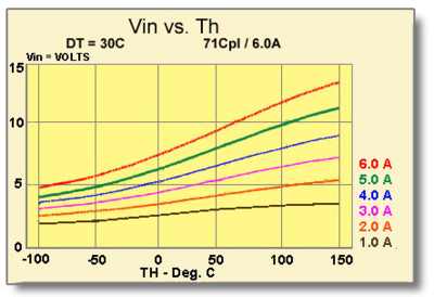
Figure (9.4) Input voltage related to input current as a function of hot side temperature for a 71-Couple, 6-Ampere Module
9.5 DESIGN EXAMPLE: To illustrate the typical design process let us present an example of a TE cooler application involving the temperature stabilization of a laser diode. The diode, along with related electronics, is to be mounted in a DIP Kovar housing and must be maintained at a temperature of 25°C. With the housing mounted on the system circuit board, tests show that the housing has a thermal resistance of 6°C/watt. The laser electronics dissipate a total of 0.5 watts and the design maximum ambient temperature is 35°C.
It is necessary to select a TE cooling module that not only will have sufficient cooling capacity to maintain the proper temperature, but also will meet the dimensional requirements imposed by the housing. An 18-couple, 1.2 ampere TE cooler is chosen initially because it does have compatible dimensions and also appears to have appropriate performance characteristics. Performance graphs for this module will be used to derive relevant parameters for making mathematical calculations. To begin the design process we must first evaluate the heat sink and make an estimate of the worst-case module hot side temperature (Th). For the TE cooler chosen, the maximum input power (Pin) can be determined from Figure (9.5) at point A.
- Max. Module Input Power (Pin) = 1.2 amps x 2.4 volts = 2.9 watts
- Max. Heat Input to the Housing = 2.9 watts + 0.5 watts = 3.4 watts
- Housing Temperature Rise = 3.4 watts x 6°C/watt = 20.4°C
- Max. Housing Temperature (T,) = 35°C ambient + 20.4°C rise = 55.4°C Since the hot side temperature (Th) of 55.4°C is reasonably close to the available Tin = 50°C performance graphs, these graphs may be used to determine thermal performance with very little error.
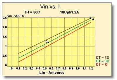
Figure (9.5) Vin vs. I graph for an 18-Couple, I.2 Ampere Module
Now that we have established the worst-case Th value it is possible to assess module performance.
Module Temperature Differential (DT) = Th — Tc = 55.4 — 25 = 30°C
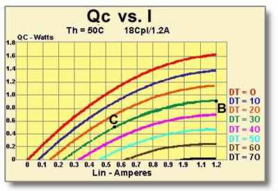
Figure (9.6) Qc vs. I graph for an 18-Couple, 1.2 Ampere Module
From Figure (9.6) it can be seen that the maximum heat pumping rate (Qc) for DT=30 occurs at point B and is approximately 0.9 watts. Since a Qc of only 0.5 watts is needed, we can follow the DT=30 line down until it intersects the 0.5 watt line marked as point C. By extending a line downward from point C to the x-axis, we can see that an input current (I) of approximately 0.55 amperes will provide the required cooling performance. Referring back to the Vin vs. I graph in Figure (9.5), a current of 0.55 amperes, marked as point D, requires a voltage (Vin) of about 1.2 volts. We now have to repeat our analysis because the required input power is considerably lower than the value used for our initial calculation. The new power and temperature values will be:
- Max. Module Input Power (Pin) = 0.55 amps x 1.2 volts = 0.66 watts
- Max. Heat Input to the Housing = 0.66 watts + 0.50 watts = 1.16 watts
- Housing Temperature Rise = 1.16 watts x 6°C/watt = 7°C
- Max. Housing Temperature (Th) = 35°C ambient + 7°C rise = 42°C
Module Temperature Differential (DT) = Th-Tc = 42°C-25°C = 17°C
It can be seen that because we now have another new value for Th it will be necessary to continue repeating the steps outlined above until a stable condition is obtained. Note that calculations usually are repeated until the difference in the Th values from successive calculations is quite small (often less that 0.1°C for good accuracy). There is no reason to present the repetitive calculations here but we can conclude that the selected 18-couple TE module will function very well in this application. This analysis clearly shows the importance of the heat sink in any thermoelectric cooling application.
9.6 USE OF MULTIPLE MODULES: Relatively large thermoelectric cooling applications may require the use of several individual modules in order to obtain the required rate of heat removal. For such applications, TE modules normally are mounted thermally in parallel and connected electrically in series. An electrical series-parallel connection arrangement may also be used advantageously in certain instances. Because heat sink performance becomes increasingly important as power levels rise, be sure that the selected heat sink is adequate for the application.